
In Part 2, a server trained a model across three hospitals by averaging their updates, weighted by how much data each one had. That rule, FedAvg, is the default in almost every federated system, and for good reason: it is simple, cheap and often good enough.
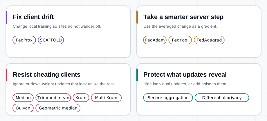
It is also the part of the system that decides what the model becomes. The aggregator, the rule that turns many client updates into one new model, is where a federated system copes with uneven data, resists clients that cheat, and limits what the updates give away. This post goes through the main alternatives to FedAvg, what each one changes, and what each one costs.
Every number and chart below comes from a small simulation you can run yourself, in plain Python and numpy, in a few seconds. The code is in four short blocks; run them one after another in the same file or notebook.
The test bed: ten very different hospitals
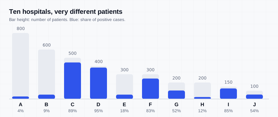
Part 2 used three hospitals that all saw the same pattern. Real federations are messier, so this time there are ten, and they differ in the way that causes real trouble: some see almost only healthy patients, others almost only sick ones. Each also has its own scanner, which shifts all its measurements slightly. The model is a small classifier, logistic regression with five inputs, that predicts whether a patient is positive.
import numpy as np

rng = np.random.default_rng(0)
SIGNAL = np.array([1.0, 0.6, 0.4, 0.0, 0.0])   # what separates sick from healthy

def make_site(n, positive_rate, offset):
    """One hospital: n patients, its own share of positive cases, its own scanner offset."""
    y = (rng.random(n) < positive_rate).astype(float)
    x = rng.normal(0, 1, (n, 5)) + np.outer(2 * y - 1, SIGNAL) + offset
    return x, y

sizes = [800, 600, 500, 400, 300, 300, 200, 200, 150, 100]
positive = [0.05, 0.10, 0.90, 0.95, 0.20, 0.80, 0.50, 0.15, 0.85, 0.50]
sites = [make_site(n, p, rng.normal(0, 0.5, 5)) for n, p in zip(sizes, positive)]
x_test, y_test = make_site(3000, 0.5, 0)       # a balanced test set

# The model: logistic regression, 6 numbers (5 weights and a bias)
def predict(w, x):
    z = np.clip(x @ w[:-1] + w[-1], -30, 30)
    return 1 / (1 + np.exp(-z))

def accuracy(w):
    return np.mean((predict(w, x_test) > 0.5) == y_test)

def gradient(w, x, y):
    err = predict(w, x) - y
    return np.append(x.T @ err / len(y), err.mean())

def local_training(w, x, y, steps=5, lr=0.5, mu=0.0, correction=0.0):
    start = w.copy()
    for _ in range(steps):
        w = w - lr * (gradient(w, x, y) + mu * (w - start) + correction)
    return w

def fedavg(models, n):
    return sum(m * k for m, k in zip(models, n)) / sum(n)
Problem 1: client drift
When every site trains for many steps before sending its update, each local model walks a long way towards what is best for that site. A site with 95% positive cases learns to say “positive” a little too readily; a site with 4% learns the opposite. Averaging these walks does not give the same result as training on all the data together. The federated model settles somewhere else, and where it settles depends on settings such as the number of local steps, not only on the data. This is called client drift.
There are two well-known fixes, both of which change what happens on the clients:
- FedProx adds a penalty to each site’s training for moving too far from the global model it started from. The site still learns from its data, but on a leash. In the code, that is the
mu * (w - start)term. - SCAFFOLD estimates, for every site, how its updates usually differ from everyone else’s, and subtracts that difference during local training. Each site gets its own correction, and the server keeps a shared one.
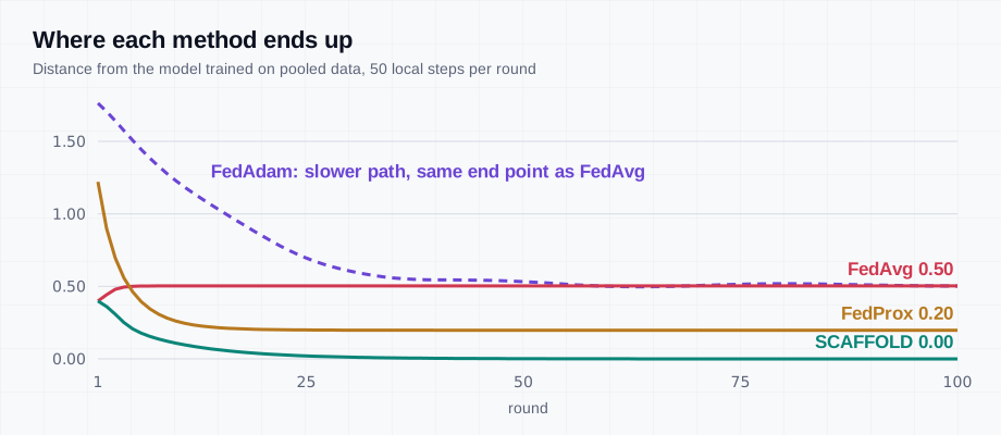
A third family changes only the server. FedAdam, FedYogi and FedAdagrad treat the averaged change as a gradient and feed it to an optimiser of the same name, with momentum and a step size per parameter. The block below compares all four, with 50 local steps per round, by measuring how far each one ends up from the model trained on pooled data.
# The target: the model we would get if all the data were pooled
x_all = np.concatenate([x for x, _ in sites])
y_all = np.concatenate([y for _, y in sites])
pooled = np.zeros(6)
for _ in range(3000):
    pooled = pooled - 0.5 * gradient(pooled, x_all, y_all)

def run(method, rounds=100, steps=50):
    w = np.zeros(6)
    c, c_site = np.zeros(6), [np.zeros(6) for _ in sites]     # SCAFFOLD only
    m, v = np.zeros(6), np.zeros(6)                            # FedAdam only
    gaps = []
    for _ in range(rounds):
        if method == "scaffold":
            models = [local_training(w, x, y, steps, correction=c - ci)
                      for (x, y), ci in zip(sites, c_site)]
            new_c = [ci - c + (w - m) / (steps * 0.5) for ci, m in zip(c_site, models)]
            c = c + fedavg([a - b for a, b in zip(new_c, c_site)], sizes)
            c_site = new_c
        else:
            mu = 0.3 if method == "fedprox" else 0.0
            models = [local_training(w, x, y, steps, mu=mu) for x, y in sites]
        if method == "fedadam":                  # the average becomes a "gradient"
            step = fedavg(models, sizes) - w
            m = 0.9 * m + 0.1 * step
            v = 0.99 * v + 0.01 * step**2
            w = w + 0.03 * m / (np.sqrt(v) + 1e-3)
        else:
            w = fedavg(models, sizes)
        gaps.append(np.linalg.norm(w - pooled))
    return w, gaps

for method in ("fedavg", "fedprox", "scaffold", "fedadam"):
    w, gaps = run(method)
    print(f"{method:<9} distance to pooled model: round 1 {gaps[0]:.2f}, "
          f"round 10 {gaps[9]:.2f}, round 100 {gaps[-1]:.2f}  accuracy {accuracy(w):.3f}")
fedavg    distance to pooled model: round 1 0.40, round 10 0.50, round 100 0.50  accuracy 0.879
fedprox   distance to pooled model: round 1 1.22, round 10 0.26, round 100 0.20  accuracy 0.872
scaffold  distance to pooled model: round 1 0.40, round 10 0.11, round 100 0.00  accuracy 0.869
fedadam   distance to pooled model: round 1 1.76, round 10 1.23, round 100 0.50  accuracy 0.879
Three lessons are in this small example.
- SCAFFOLD lands on the pooled model (to two decimals), and FedProx gets most of the way there. FedProx starts slower, because the leash holds the first rounds back.
- A server optimiser changes the path, not the destination. FedAdam ends where FedAvg ends. Its strengths lie elsewhere: noisy updates, only some clients taking part in each round, and models whose parameters need very different step sizes (Reddi et al., 2021). It also brings a server learning rate that has to be tuned.
- Distance is not the same as accuracy. In a model this small, the drifted FedAvg model even scores marginally higher on our balanced test set, because the drift happens to lean towards balance. Drift means the result depends on training settings instead of on the data, which makes it hard to reason about. In deep networks it usually costs accuracy too.
SCAFFOLD’s precision has a price: every site keeps an extra correction, and every round sends it back and forth, roughly doubling the traffic. Clients that drop out or join late also complicate it; how to make late-joining clients useful quickly is the problem our work on FedRecall looks at.
Problem 2: clients that cheat
FedAvg trusts every client. A client that sends a bad update, whether from a bug, broken hardware or on purpose, pulls the average with exactly as much force as its weight allows. In the next experiment, hospitals B and E, a quarter of all patients, cheat. They train on deliberately flipped labels, calling healthy patients sick and sick patients healthy, and they multiply their update by three to make it count for more.
It helps to look at what the server actually receives. The plot below shows the ten models sent in the first round, using two of each model’s six numbers.
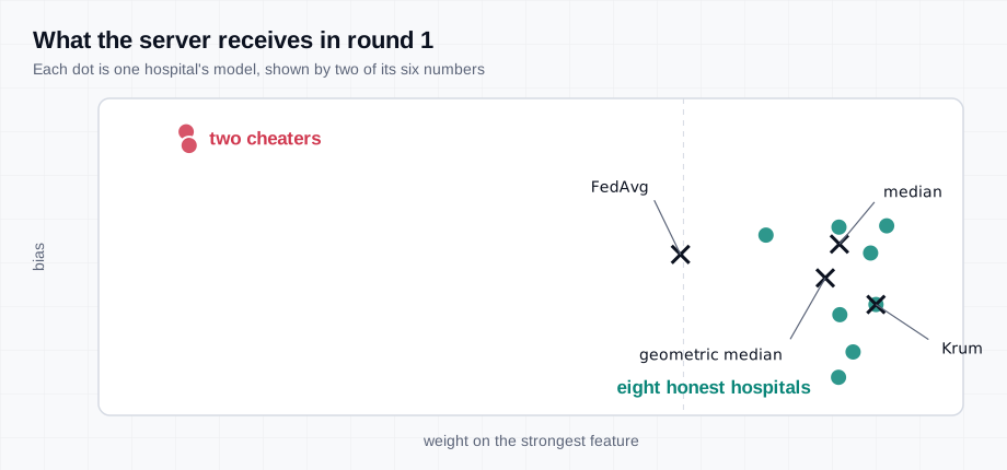
Robust aggregators look at the updates before combining them and limit the influence of the ones that look unlike the rest:
- Coordinate-wise median: for each of the model’s numbers, take the median across clients instead of the mean.
- Trimmed mean: for each number, drop the highest and lowest values (here 20% at each end) and average the rest.
- Krum: give each update a score based on how close it is to its nearest neighbours, and keep the single most typical one. Multi-Krum keeps the most typical several and averages them.
- Geometric median: the single point with the smallest total distance to all updates, found by a short iterative calculation (Weiszfeld’s algorithm).
def median(models, n):
    return np.median(models, axis=0)

def trimmed_mean(models, n, cut=0.2):
    k = int(len(models) * cut)
    return np.sort(models, axis=0)[k:len(models) - k].mean(axis=0)

def krum(models, n, f=2, keep=1):
    m = np.array(models)
    dist = ((m[:, None] - m[None]) ** 2).sum(-1)
    score = [np.sort(d)[1:len(m) - f - 1].sum() for d in dist]   # closeness to its neighbours
    return m[np.argsort(score)[:keep]].mean(axis=0)

def multi_krum(models, n):
    return krum(models, n, keep=len(models) - 2)

def geometric_median(models, n, iters=100):
    m = np.array(models)
    z = m.mean(axis=0)
    for _ in range(iters):                                         # Weiszfeld's algorithm
        d = np.maximum(np.linalg.norm(m - z, axis=1), 1e-8)
        z = (m / d[:, None]).sum(0) / (1 / d).sum()
    return z

cheaters = {1, 4}           # hospitals B and E: 900 of the 3,550 patients

def run_attack(aggregate, attack, rounds=60):
    w = np.zeros(6)
    for _ in range(rounds):
        models = []
        for i, (x, y) in enumerate(sites):
            if attack and i in cheaters:
                m = local_training(w, x, 1 - y)        # train on flipped labels...
                m = w + 3 * (m - w)                     # ...and boost the update
            else:
                m = local_training(w, x, y)
            models.append(m)
        w = aggregate(models, sizes)
    return accuracy(w)

for name, agg in [("FedAvg", fedavg), ("Median", median), ("Trimmed mean", trimmed_mean),
                  ("Krum", krum), ("Multi-Krum", multi_krum), ("Geometric median", geometric_median)]:
    print(f"{name:<17} no attack {run_attack(agg, False):.3f}   two cheaters {run_attack(agg, True):.3f}")
FedAvg            no attack 0.870   two cheaters 0.517
Median            no attack 0.849   two cheaters 0.768
Trimmed mean      no attack 0.880   two cheaters 0.825
Krum              no attack 0.833   two cheaters 0.841
Multi-Krum        no attack 0.858   two cheaters 0.878
Geometric median  no attack 0.843   two cheaters 0.835
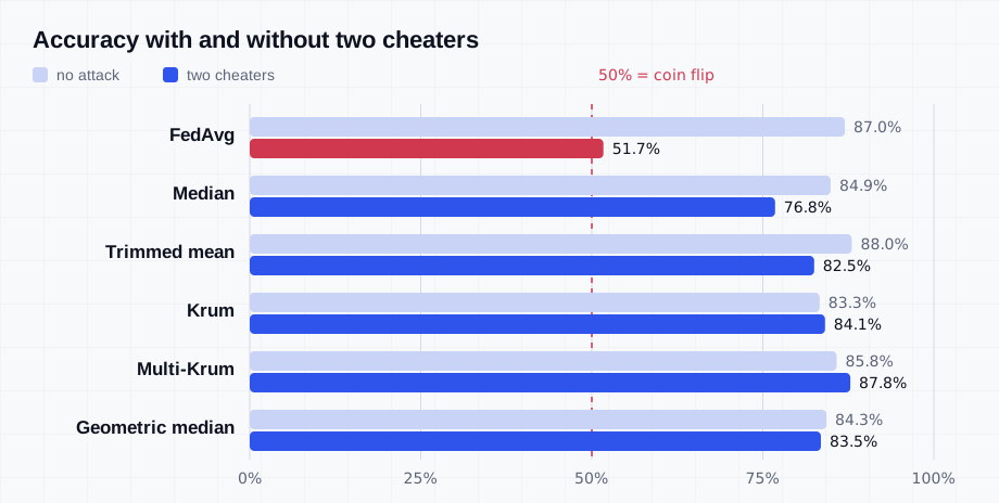
The results show both the value and the cost of robustness.
- FedAvg collapses. With two cheaters it scores 51.7%, no better than guessing.
- Every robust rule keeps a useful model, from 76.8% for the median to 87.8% for Multi-Krum.
- Robustness is not free when nobody cheats. Krum keeps a single hospital’s model and throws the other nine away, so without an attack it scores 83.3% instead of 87.0%. The median ignores how much data each hospital has. With uneven sites like these, an honest but unusual hospital looks a lot like a cheater.
- Multi-Krum does better under attack than without it. It always drops the two least typical updates. Under attack, those are the cheaters. Without one, they are honest hospitals with unusual patients.
Two practical limits are worth knowing. Robust rules need enough clients. To tolerate f cheaters, Krum needs more than 2f + 2 clients in total, and Bulyan, which combines Krum with a trimmed mean, needs at least 4f + 3. With ten clients and two cheaters, Krum works but Bulyan cannot run at all. And these rules assume cheaters are a minority that looks different. A careful attacker who stays just inside the honest cloud can still do damage.
Our own approach takes a different angle. Instead of judging updates by how typical they look, we weigh each update by how well it performs on a small, clean validation set held by the server. In experiments on chest X-rays it held off both label flipping and backdoor attacks (paper). The trade-off is that the server needs that trusted validation data.
Problem 3: updates that reveal too much
A model update is computed from private data, and research on gradient leakage (Zhu et al., 2019) has shown that individual updates can sometimes be turned back into recognisable training examples. Two tools address this, and they protect against different things.
Secure aggregation uses cryptography so that the server learns only the sum of the updates, never any single one (Bonawitz et al., 2017). It costs no accuracy. It does conflict with the previous section, though: robust aggregators need to see individual updates to spot the outliers, and secure aggregation hides exactly those. Combining the two is an active research area.
Differential privacy limits what the final model can reveal about any one participant, however the model is later used. On its own, it does not hide individual updates from the server, which is why it is often combined with secure aggregation. In its common federated form (McMahan et al., 2018), there are two steps:
- each update is clipped to a maximum size, so that no single hospital can move the model too far;
- random noise is added to the sum, scaled to that maximum size.
The privacy guarantee is summarised by a number, ε (epsilon). Lower means stronger privacy; values around 1 to 10 are typical targets in practice. Here the “individual” being protected is a whole hospital, which is the strictest form.
def run_private(noise, clip=1.0, rounds=60, seed=1):
    noise_rng = np.random.default_rng(seed)
    w = np.zeros(6)
    for _ in range(rounds):
        updates = []
        for x, y in sites:
            u = local_training(w, x, y) - w
            u = u * min(1.0, clip / np.linalg.norm(u))       # 1. clip each update
            updates.append(u)
        mean = np.mean(updates, axis=0)
        mean += noise_rng.normal(0, noise * clip / len(sites), 6)   # 2. add noise to the sum
        w = w + mean
    return accuracy(w)

def epsilon(noise, rounds=60, delta=1e-5):
    """Privacy budget for one hospital over all rounds (Rényi DP bound; lower is more private)."""
    return 2 * rounds / noise**2 + 2 * np.sqrt(2 * rounds * np.log(1 / delta)) / noise

print(f"no noise   epsilon    inf   accuracy {run_private(0):.3f}")
for noise in (1, 4, 16, 64):
    runs = [run_private(noise, seed=s) for s in range(20)]   # noise is random: average 20 runs
    print(f"noise {noise:>2}   epsilon {epsilon(noise):6.1f}   accuracy {np.mean(runs):.3f}"
          f"  (worst run {min(runs):.3f})")
no noise   epsilon    inf   accuracy 0.883
noise  1   epsilon  194.3   accuracy 0.877  (worst run 0.865)
noise  4   epsilon   26.1   accuracy 0.845  (worst run 0.686)
noise 16   epsilon    5.1   accuracy 0.755  (worst run 0.370)
noise 64   epsilon    1.2   accuracy 0.564  (worst run 0.251)
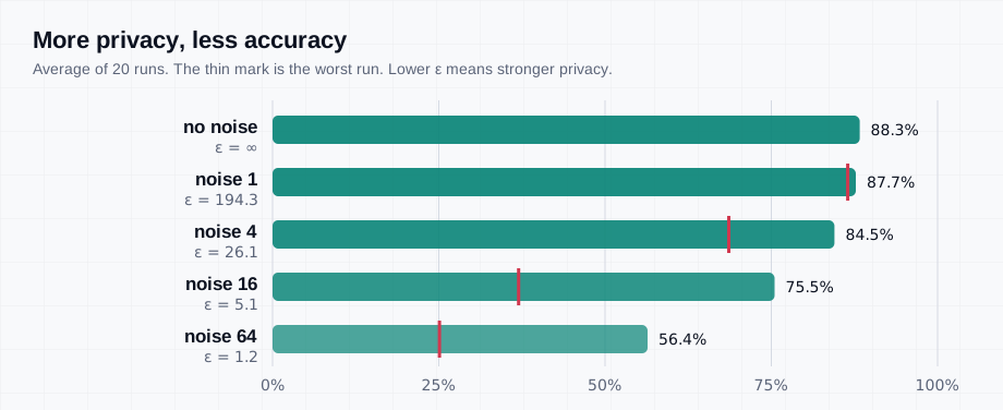
The trade-off is plain. Light noise costs almost nothing but gives a weak guarantee. A strong guarantee, ε around 1, takes the model from 88% to 56% on average. With ten hospitals there are too few updates for the noise to average out. Differential privacy at the level of whole clients works far better with hundreds or thousands of them, which is why it is used in production on phones, for example in Gboard’s keyboard models and much harder between a handful of hospitals. Between organisations it is more common to protect individual patients inside each hospital’s training, which needs much less noise.
Which aggregator when
| Situation | Start with | Watch out for |
|---|---|---|
| Similar sites, all trusted | FedAvg | Nothing. It is the baseline to beat. |
| Very different sites, many local steps | FedProx or SCAFFOLD | FedProx’s mu needs tuning; SCAFFOLD needs extra state on every client and roughly twice the traffic. |
| Noisy updates, few clients per round | FedAdam or FedYogi | A server learning rate to tune. On their own, they do not fix drift. |
| Some clients may be faulty or hostile | Trimmed mean, Multi-Krum or geometric median | They need enough clients, cost some accuracy when nobody cheats, and need to see individual updates. |
| Individual updates must stay hidden | Secure aggregation | It hides exactly what robust aggregators need to see. |
| The final model must not reveal any participant | Differential privacy | It costs accuracy, and works best with many clients. |
Two habits matter more than any single choice. First, compare against FedAvg on your own data, because the extra machinery is not always worth it. Second, look at results per site: a method that improves the average while failing the smallest hospital is not an improvement for that hospital.
What comes next
In this post, every method ran inside one Python process. In a real deployment, the aggregator runs on a server, hospitals connect over a network, and some of these choices depend on where in the system aggregation happens. That is the job of a framework. Part 4 surveys the main open-source frameworks and how to choose between them, and Part 5 will introduce Decentrai, my own framework for hierarchical federated learning, which ships 18 aggregation algorithms, including most of the ones above.
Further reading
- Li et al. (2020). Federated Optimization in Heterogeneous Networks. FedProx.
- Karimireddy et al. (2020). SCAFFOLD: Stochastic Controlled Averaging for Federated Learning.
- Reddi et al. (2021). Adaptive Federated Optimization. FedAdam, FedYogi and FedAdagrad.
- Blanchard et al. (2017). Machine Learning with Adversaries: Byzantine Tolerant Gradient Descent. Krum.
- Yin et al. (2018). Byzantine-Robust Distributed Learning: Towards Optimal Statistical Rates. Median and trimmed mean.
- El Mhamdi, Guerraoui and Rouault (2018). The Hidden Vulnerability of Distributed Learning in Byzantium. Bulyan.
- Pillutla, Kakade and Harchaoui (2022). Robust Aggregation for Federated Learning. The geometric median.
- Bonawitz et al. (2017). Practical Secure Aggregation for Privacy-Preserving Machine Learning.
- McMahan et al. (2018). Learning Differentially Private Recurrent Language Models. Differential privacy in federated learning.
Want to go further? Browse my publications on federated learning, or look at the open thesis topics if you would like to work on these problems with us.